
Date: 18 June 2026
Tag: sPH-CONF-JET-2026-01
Document: Conference Note
(Back to sPHENIX Public Results page.)
Figure 1 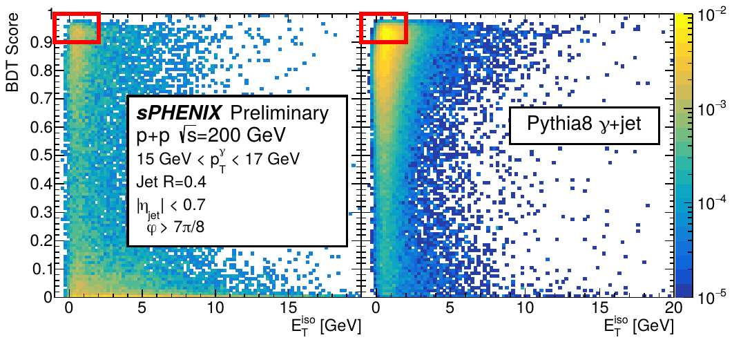
Distribution of isolation energies and BDT scores of EMCal clusters with pTγ = 15–17 GeV in p+p (left) collision data and (right) PYTHIA-8 γ-jet simulations. The band in the bottom left that exists in data but not in simulation is made of decay photons which are rejected by the BDT cut. Here, only clusters with an away-side jet, as described in the text, are plotted. The selected signal region is shown in the red box. |
Figure 2 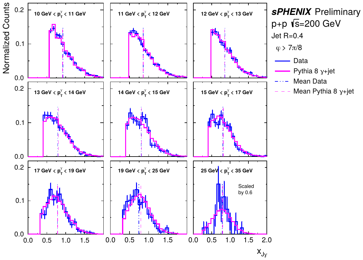
Distributions of xJγ for R = 0.4 jets, shown separately for each pTγ interval in p+p data and reconstructed-level PYTHIA-8 simulation. Statistical uncertainties on the data are shown as error bars, meanwhile the statistical uncertainties on the simulation are significantly smaller and not shown. The dashed and dash-dotted lines indicate the mean xJγ values. |
Figure 3 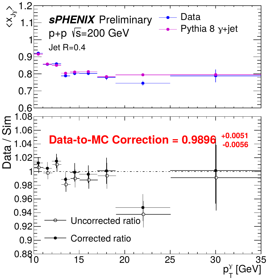
The top panel shows the ⟨xJγ⟩ as a function of pTγ for R = 0.4 jets in data and PYTHIA-8 simulation. The bottom panel shows the ratio of ⟨xJγ⟩ between data and simulation before and after Data-to-MC JES correction. A dashed line is drawn at 1 for a reference, and the points are slightly offset for visual clarity. The correction parameter a and the associated statistical uncertainty are quoted. |
Figure 4 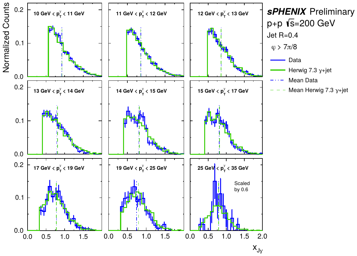
Distributions of xJγ for R = 0.4 jets, shown separately for each pTγ interval in p+p data and reconstructed-level HERWIG-7.3 simulation. Statistical uncertainties on the data are shown as error bars, meanwhile the statistical uncertainties on the simulation are significantly smaller and not shown. The dashed and dash-dotted lines indicate the mean xJγ values. |
Figure 5 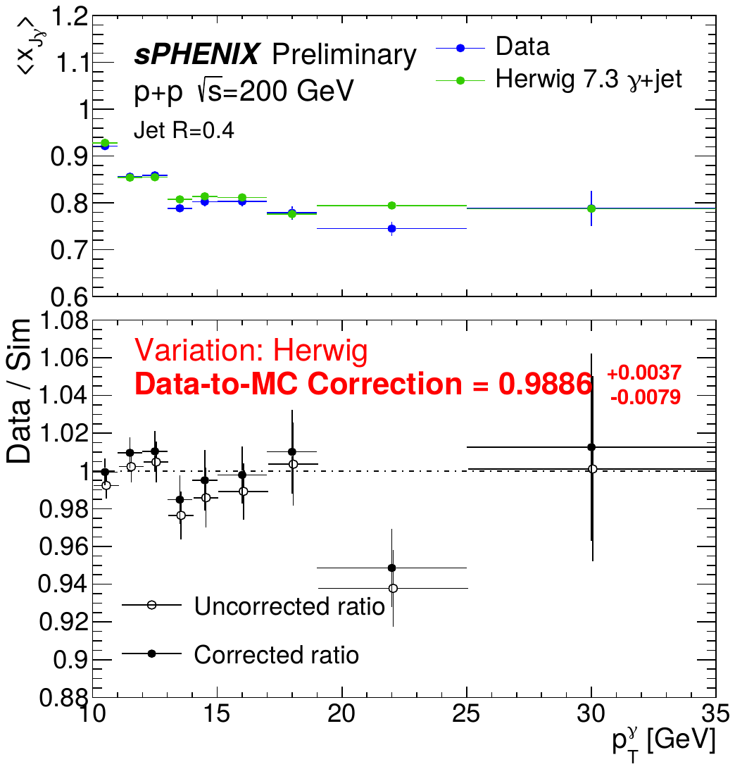
The top panel shows the ⟨xJγ⟩ as a function of pTγ for R = 0.4 jets in data and HERWIG-7.3 simulation. The bottom panel shows the ratio of ⟨xJγ⟩ between data and simulation before and after Data-to-MC JES correction. A dashed line is drawn at 1 for a reference, and the points are slightly offset for visual clarity. The correction parameter a and the associated statistical uncertainty are quoted. |
Figure 6 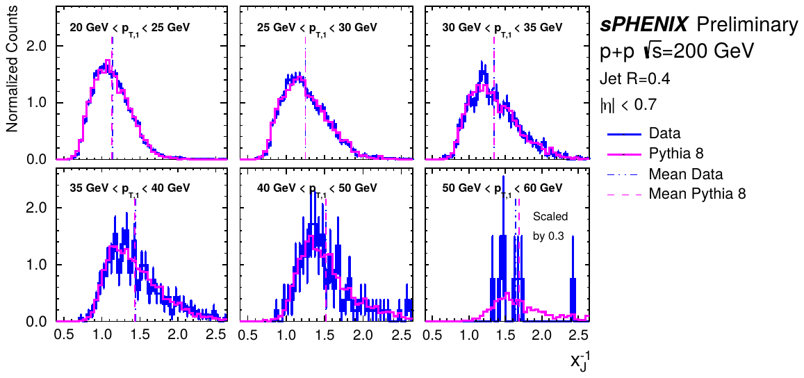
Distributions of multijet xJ−1 for the MBM analysis of R = 0.4 jets, shown for each pT,1 interval in p+p data and reconstructed-level PYTHIA-8 simulation. Statistical uncertainties on the data are shown as error bars, meanwhile the statistical uncertainties on the simulation are significantly smaller and not shown. |
Figure 7 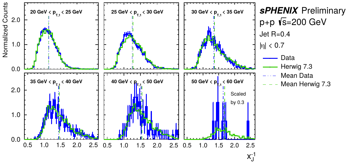
Distributions of multijet xJ−1 for the MBM analysis of R = 0.4 jets, shown separately for each pT,1 interval in p+p data and reconstructed-level HERWIG-7.3 simulation. Statistical uncertainties on the data are shown as error bars, meanwhile the statistical uncertainties on the simulation are significantly smaller and not shown. |
Figure 8 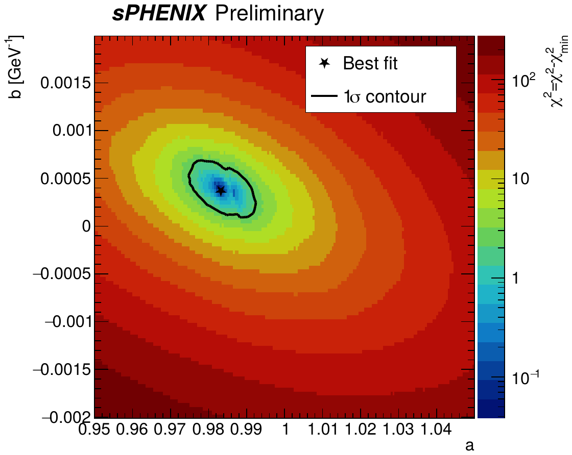
Δχ2 distribution as a function of the two global fit parameters, a and b. A black star shows the minimum χ2 value. The black contour corresponds to the one standard deviation confidence region based on statistical uncertainties only. |
Figure 9 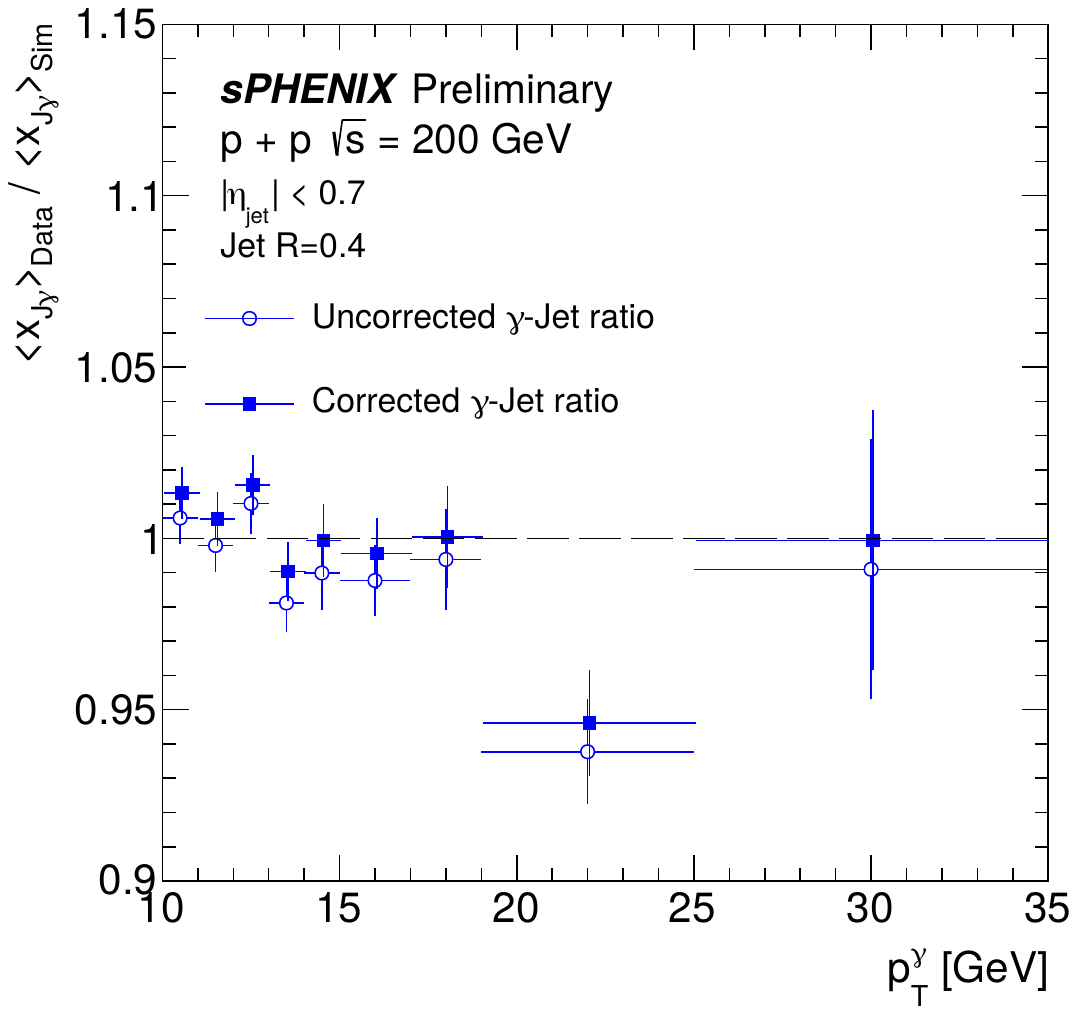
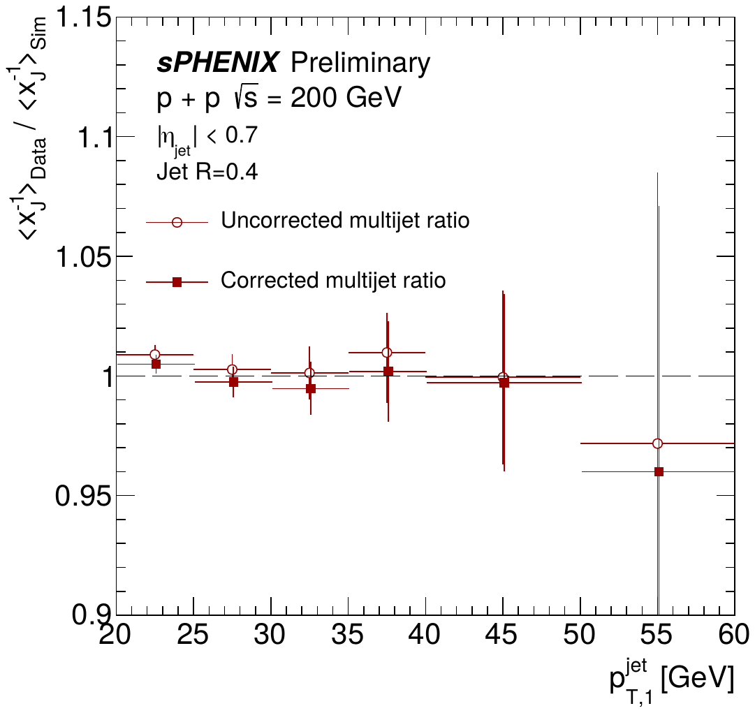
Comparison of data–simulation agreement (left) for the γ-jet analysis and (right) the MBM analysis, shown as the ratio of ⟨xJγ⟩ and ⟨xJ−1⟩, respectively, between data and simulation. The open and closed points correspond to the values before and after the application of the optimized Data-to-MC JES correction. A dashed line is drawn at 1 for a reference, and the points are slightly offset for visual clarity. |
Figure 10 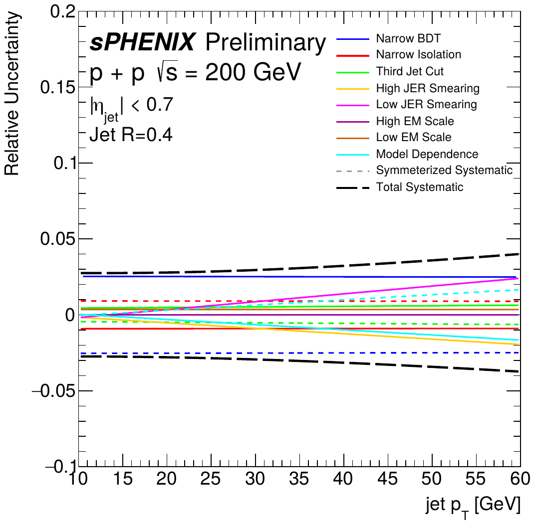
Summary of systematic uncertainties on the global JES correction function. The relative difference of the best-fit function to the nominal function is shown under the application of different systematic variations. All systematic uncertainty variations are symmetrized, except the separate high and low JER smearing and electromagnetic scaling, and then added in quadrature. The black dashed line shows the total systematic uncertainty. |
Figure 11 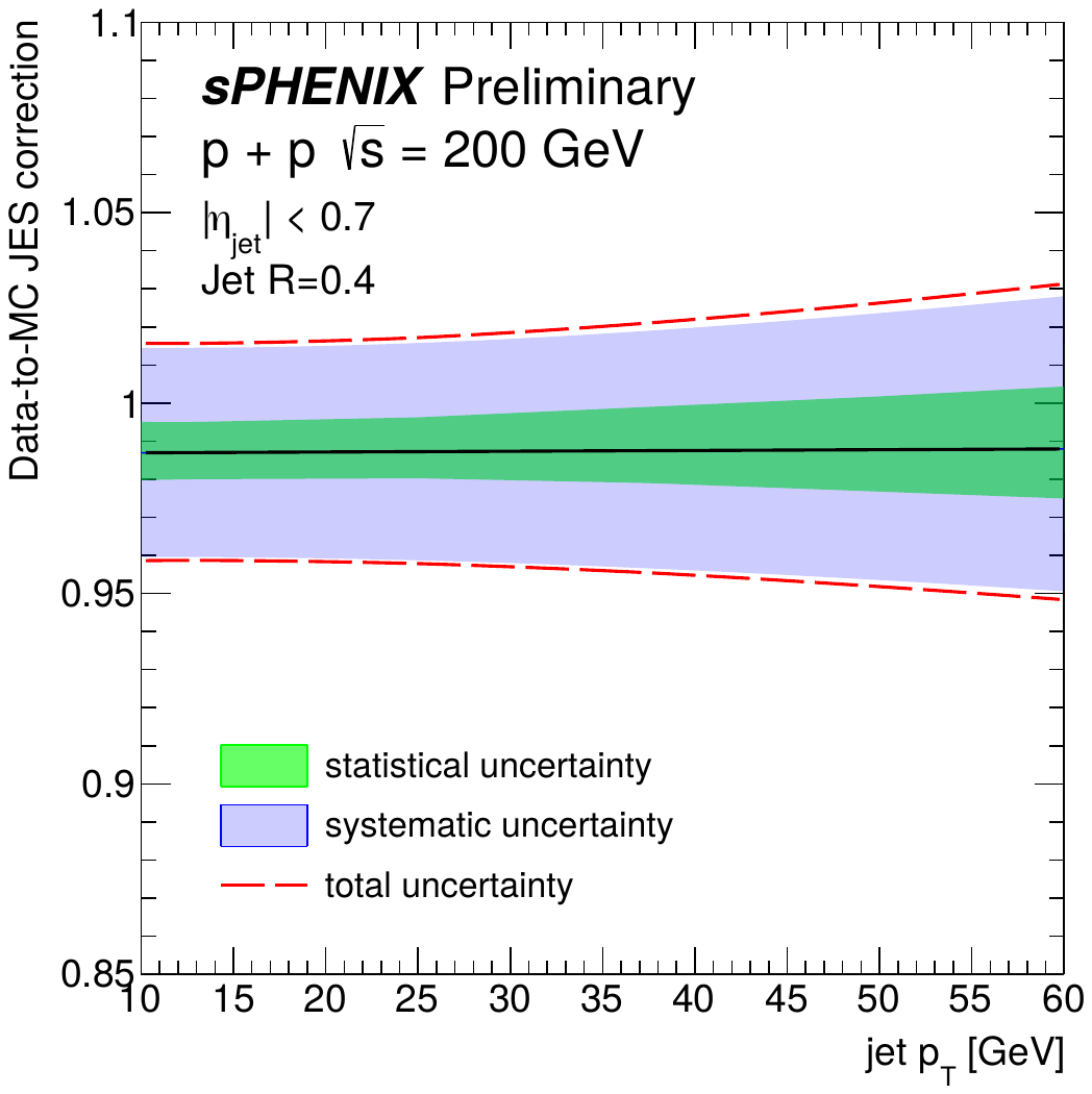
Global Data-to-MC JES correction as a function of calorimeter jet pT, shown here for R = 0.4 jets. The black line is the central value. The green and blue shaded bands show the total statistical and systematic uncertainty, and the dashed red line shows the total uncertainty. |
Figure 12 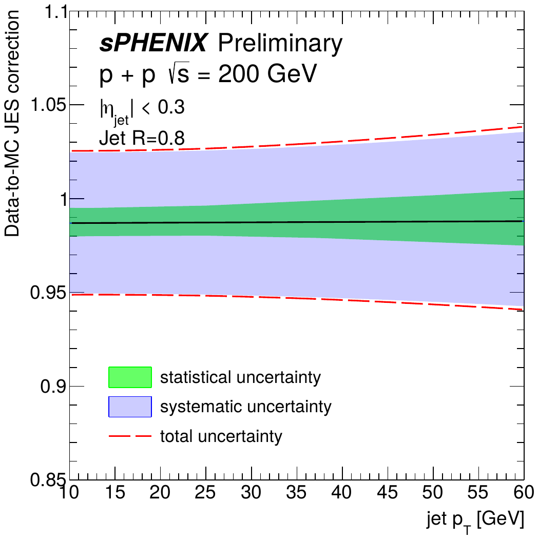
Global Data-to-MC JES correction as a function of calorimeter jet pT shown for R = 0.8 jets. The black line is the central value. The green and blue shaded bands show the total statistical and systematic uncertainty, and the dashed red line shows the total uncertainty. |
Figure 13 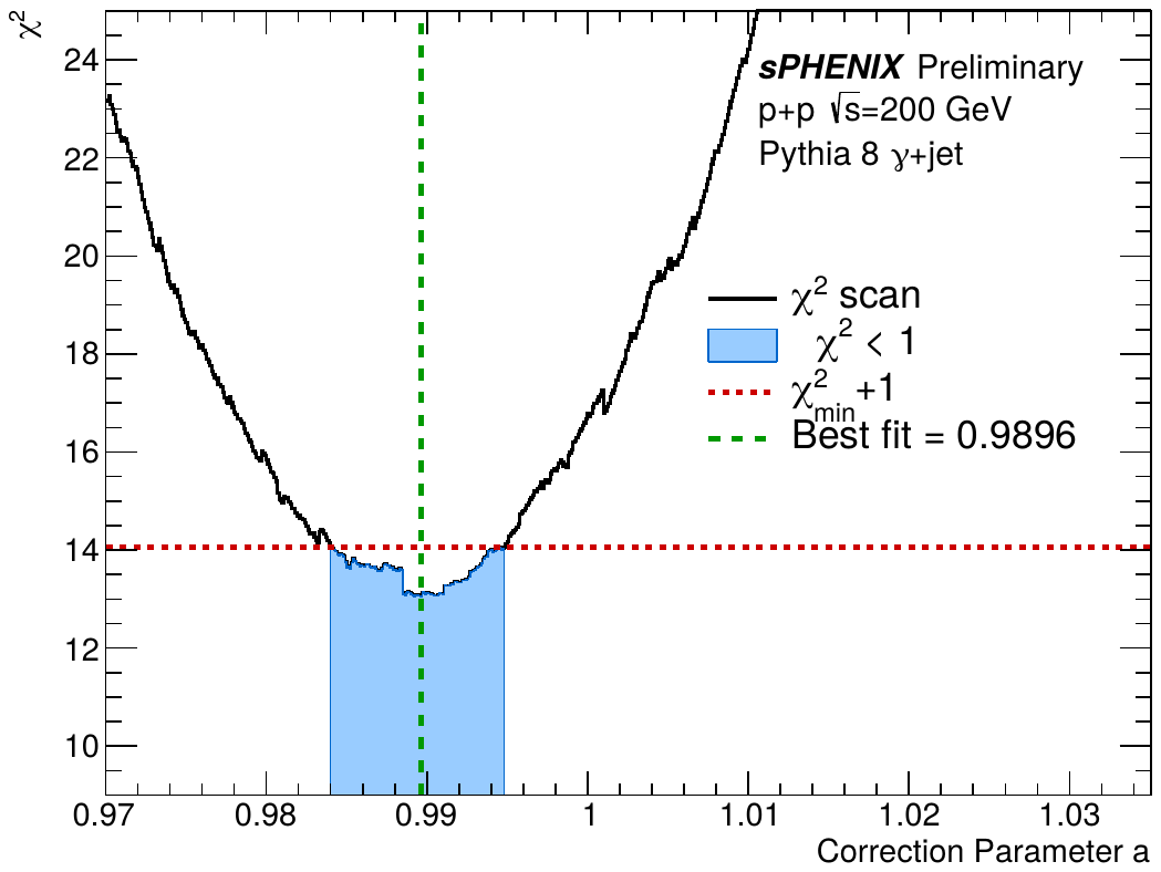
A visualization of the one-dimensional grid scan used for the γ-jet results. The Data-to-MC JES correction using the γ-jet results alone assumes there is no pT dependence, and the correction takes the form C(pT) = a, where the corrected jet in data is equal to pTjet/C. The statistical uncertainties on the correction are determined by grid values for which χ2 < χ2min + 1. |
Figure 14 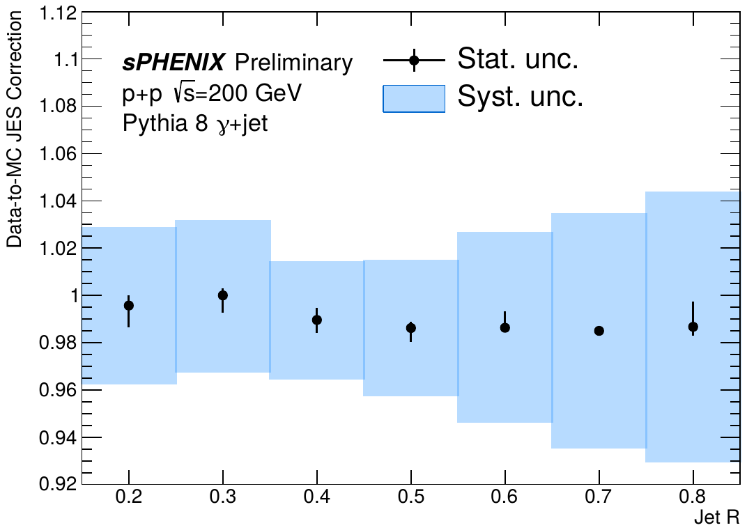
The Data-to-MC JES correction values from the γ-jet only constraint. The vertical error bars are the asymmetric statistical uncertainties, and the boxes are the total systematic uncertainties. Within uncertainties, there is no jet radius dependence to the Data-to-MC JES correction. |