Date: 15 June 2026
Tag: sPH-JET-2026-01
Document: arXiv preprint
(Back to sPHENIX Public Results page.)
Figure 1 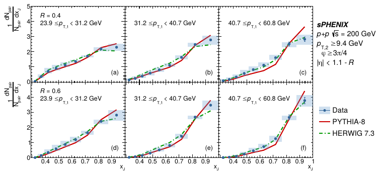
Unfolded xJ distributions for R = 0.4 (upper row — panels (a)-(c)) and R = 0.6 (lower row — panels (d)-(f)) jets in three pT,1 selections. Vertical bars indicate statistical uncertainties, and boxes indicate systematic uncertainties. Data are compared to particle-level PYTHIA (Detroit tune) and HERWIG (Nashville tune) calculations. |
Figure 2 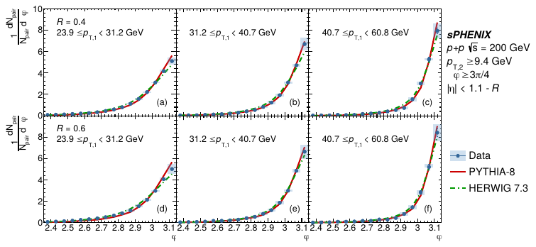
Corrected Δφ distributions for R = 0.4 (upper row — panels (a)-(c)) and R = 0.6 (lower row — panels (d)-(f)) jets in three pT,1 selections. Vertical bars indicate statistical uncertainties, and boxes indicate systematic uncertainties. Data are compared to particle-level PYTHIA (Detroit tune) and HERWIG (Nashville tune) calculations. |
Figure 3 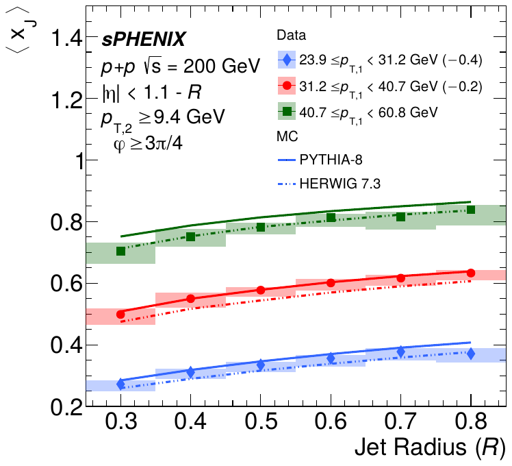
Mean xJ, ⟨xJ⟩ (top) and σ(Δφ) (bottom) as a function of jet radius R for the three pT,1 selections. In the top panel, the different pT,1 selections are shifted for clarity. Vertical bars indicate statistical uncertainties, and boxes indicate systematic uncertainties. Data are compared to PYTHIA (Detroit tune) and HERWIG (Nashville tune) calculations. |
Figure 4 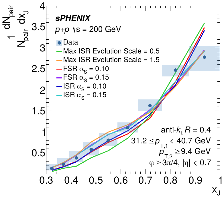
xJ distribution for R = 0.4 jets in the 31.2 ≤ pT,1 < 40.7 GeV selection. The data points are shown with systematic uncertainties, along with the distributions from PYTHIA-8 configured with minimum/maximum values of parameters sensitive to the description of ISR and FSR modeling at the LHC, holding other parameters fixed. |
Figure 5 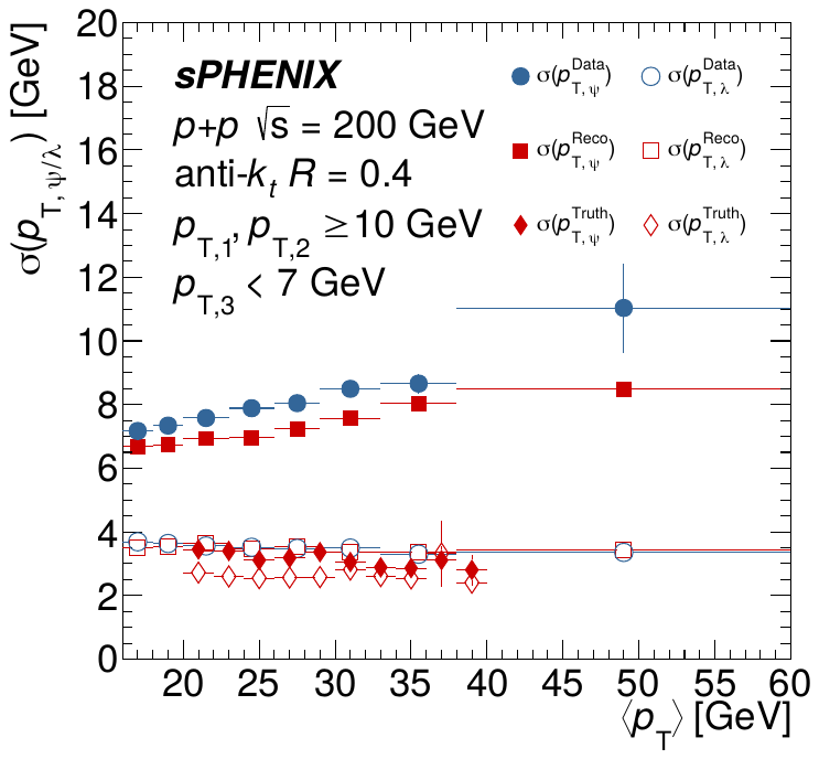
Widths σ(pT,ψ) (filled markers) and σ(pT,λ) (open markers) from the bisector method as a function of ⟨pT⟩ for R = 0.4 jets, shown for generator-level PYTHIA (diamonds), reconstructed-level PYTHIA (squares), and data (circles). |
Figure 6 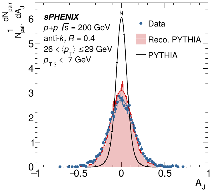
Dijet asymmetry, AJ, distributions for R = 0.4 jets in an example ⟨pT⟩ bin with a third-jet veto threshold of 7 GeV, shown for generator-level PYTHIA (black), reconstructed-level PYTHIA (red), and data (blue). The curves show Gaussian fits to the distributions. |
Figure 7 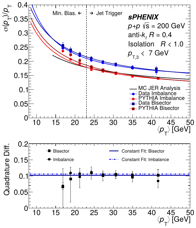
Top: relative jet pT resolution, σ(pT)/pT, for R = 0.4 jets as a function of ⟨pT⟩, shown in data (blue) and PYTHIA simulation (red) for the bisector (squares) and dijet imbalance (circles) methods. Fits to the curves of the form C ⊕ S/√pT ⊕ N/pT are overlaid, as well as the JER determined in simulation as a function of jet pT (black line). Bottom: quadrature difference of the relative resolution between data and simulation, quantifying the additional smearing applied in the measurement. |
Figure 8 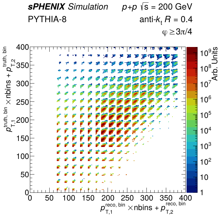
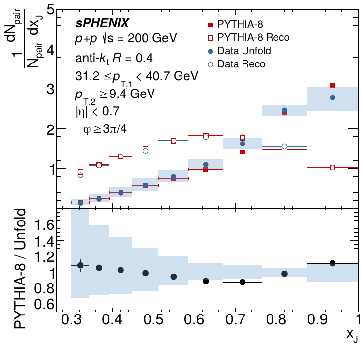
Left: Response matrix for R = 0.4 jets showing the association between truth- and reconstructed-level dijet (pT,1, pT,2) values in PYTHIA simulation. Right: The top panel shows example xJ distributions from data at the reconstructed level before unfolding (open blue circles) and after unfolding (filled blue circles) in data, and at the particle (filled red squares) and reconstructed (open red squares) levels in PYTHIA, for R = 0.4 jets in the 31.2 ≤ pT,1 < 40.7 GeV selection. The bottom panel shows the ratio of the particle-level PYTHIA to the unfolded data. In both panels, the shaded bands denote the total systematic uncertainty on the unfolded data measurement. |
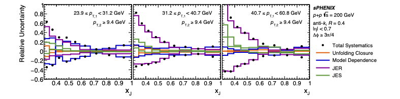
Additional Figures 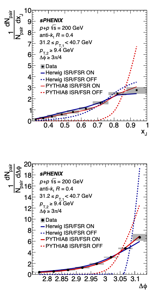
|